import java.util.ArrayList;
import java.util.List;
import java.util.Random;
import org.opencv.core.Core;
import org.opencv.core.CvType;
import org.opencv.core.Mat;
import org.opencv.core.MatOfPoint;
import org.opencv.core.Point;
import org.opencv.core.Scalar;
import org.opencv.highgui.HighGui;
import org.opencv.imgcodecs.Imgcodecs;
import org.opencv.imgproc.Imgproc;
class ImageSegmentation {
public void run(
String[] args) {
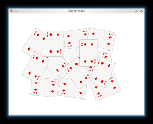
String filename = args.length > 0 ? args[0] :
"../data/cards.png";
Mat srcOriginal = Imgcodecs.imread(filename);
if (srcOriginal.empty()) {
System.err.println("Cannot read image: " + filename);
System.exit(0);
}
HighGui.imshow("Source Image", srcOriginal);
Mat src = srcOriginal.
clone();
byte[] srcData = new byte[(int) (src.total() * src.channels())];
src.get(0, 0, srcData);
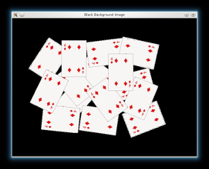
for (int i = 0; i < src.rows(); i++) {
for (int j = 0; j < src.cols(); j++) {
if (srcData[(i * src.cols() + j) * 3] == (byte) 255 && srcData[(i * src.cols() + j) * 3 + 1] == (byte) 255
&& srcData[(i * src.cols() + j) * 3 + 2] == (byte) 255) {
srcData[(i * src.cols() + j) * 3] = 0;
srcData[(i * src.cols() + j) * 3 + 1] = 0;
srcData[(i * src.cols() + j) * 3 + 2] = 0;
}
}
}
src.put(0, 0, srcData);
HighGui.imshow("Black Background Image", src);
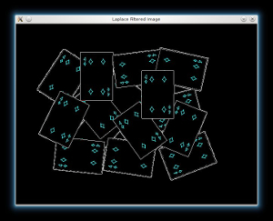
Mat kernel = new Mat(3, 3, CvType.CV_32F);
float[] kernelData = new float[(int) (kernel.total() * kernel.channels())];
kernelData[0] = 1; kernelData[1] = 1; kernelData[2] = 1;
kernelData[3] = 1; kernelData[4] = -8; kernelData[5] = 1;
kernelData[6] = 1; kernelData[7] = 1; kernelData[8] = 1;
kernel.put(0, 0, kernelData);
Mat imgLaplacian = new Mat();
Imgproc.filter2D(src, imgLaplacian, CvType.CV_32F, kernel);
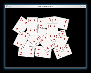
Mat sharp = new Mat();
src.convertTo(sharp, CvType.CV_32F);
Mat imgResult = new Mat();
Core.subtract(sharp, imgLaplacian, imgResult);
imgResult.convertTo(imgResult, CvType.CV_8UC3);
imgLaplacian.convertTo(imgLaplacian, CvType.CV_8UC3);
HighGui.imshow("New Sharped Image", imgResult);
Mat bw = new Mat();
Imgproc.cvtColor(imgResult, bw, Imgproc.COLOR_BGR2GRAY);
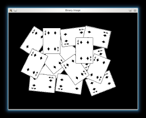
Imgproc.threshold(bw, bw, 40, 255, Imgproc.THRESH_BINARY | Imgproc.THRESH_OTSU);
HighGui.imshow("Binary Image", bw);
Mat dist = new Mat();
Imgproc.distanceTransform(bw, dist, Imgproc.DIST_L2, 3);
Core.normalize(dist, dist, 0.0, 1.0, Core.NORM_MINMAX);
Mat distDisplayScaled = new Mat();
Core.multiply(dist,
new Scalar(255), distDisplayScaled);
Mat distDisplay = new Mat();
distDisplayScaled.convertTo(distDisplay, CvType.CV_8U);
HighGui.imshow("Distance Transform Image", distDisplay);
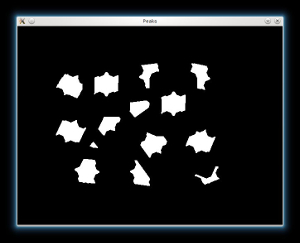
Imgproc.threshold(dist, dist, 0.4, 1.0, Imgproc.THRESH_BINARY);
Mat kernel1 = Mat.
ones(3, 3, CvType.CV_8U);
Imgproc.dilate(dist, dist, kernel1);
Mat distDisplay2 = new Mat();
dist.convertTo(distDisplay2, CvType.CV_8U);
Core.multiply(distDisplay2,
new Scalar(255), distDisplay2);
HighGui.imshow("Peaks", distDisplay2);
Mat dist_8u = new Mat();
dist.convertTo(dist_8u, CvType.CV_8U);
List<MatOfPoint> contours = new ArrayList<>();
Mat hierarchy = new Mat();
Imgproc.findContours(dist_8u, contours, hierarchy, Imgproc.RETR_EXTERNAL, Imgproc.CHAIN_APPROX_SIMPLE);
Mat markers = Mat.
zeros(dist.size(), CvType.CV_32S);
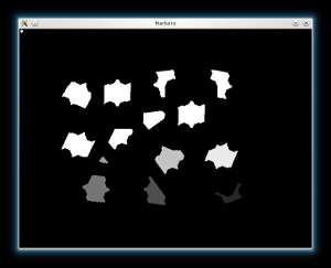
for (int i = 0; i < contours.size(); i++) {
Imgproc.drawContours(markers, contours, i,
new Scalar(i + 1), -1);
}
Mat markersScaled = new Mat();
markers.convertTo(markersScaled, CvType.CV_32F);
Core.normalize(markersScaled, markersScaled, 0.0, 255.0, Core.NORM_MINMAX);
Imgproc.circle(markersScaled,
new Point(5, 5), 3,
new Scalar(255, 255, 255), -1);
Mat markersDisplay = new Mat();
markersScaled.convertTo(markersDisplay, CvType.CV_8U);
HighGui.imshow("Markers", markersDisplay);
Imgproc.circle(markers,
new Point(5, 5), 3,
new Scalar(255, 255, 255), -1);
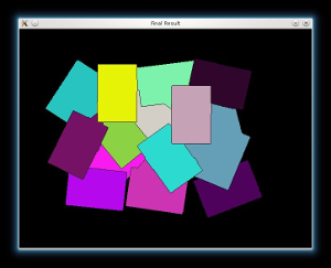
Imgproc.watershed(imgResult, markers);
Mat mark = Mat.
zeros(markers.size(), CvType.CV_8U);
markers.convertTo(mark, CvType.CV_8UC1);
Core.bitwise_not(mark, mark);
Random rng = new Random(12345);
List<Scalar> colors = new ArrayList<>(contours.size());
for (int i = 0; i < contours.size(); i++) {
int b = rng.nextInt(256);
int g = rng.nextInt(256);
int r = rng.nextInt(256);
colors.add(
new Scalar(b, g, r));
}
Mat dst = Mat.
zeros(markers.size(), CvType.CV_8UC3);
byte[] dstData = new byte[(int) (dst.total() * dst.channels())];
dst.get(0, 0, dstData);
int[] markersData = new int[(int) (markers.total() * markers.channels())];
markers.get(0, 0, markersData);
for (int i = 0; i < markers.rows(); i++) {
for (int j = 0; j < markers.cols(); j++) {
int index = markersData[i * markers.cols() + j];
if (index > 0 && index <= contours.size()) {
dstData[(i * dst.cols() + j) * 3 + 0] = (byte) colors.get(index - 1).val[0];
dstData[(i * dst.cols() + j) * 3 + 1] = (byte) colors.get(index - 1).val[1];
dstData[(i * dst.cols() + j) * 3 + 2] = (byte) colors.get(index - 1).val[2];
} else {
dstData[(i * dst.cols() + j) * 3 + 0] = 0;
dstData[(i * dst.cols() + j) * 3 + 1] = 0;
dstData[(i * dst.cols() + j) * 3 + 2] = 0;
}
}
}
dst.put(0, 0, dstData);
HighGui.imshow("Final Result", dst);
HighGui.waitKey();
System.exit(0);
}
}
public class ImageSegmentationDemo {
public static void main(
String[] args) {
System.loadLibrary(Core.NATIVE_LIBRARY_NAME);
new ImageSegmentation().run(args);
}
}


 1.8.13